TrajAnalytics
A Cloud Visual Analytics Software
Overview#back to top
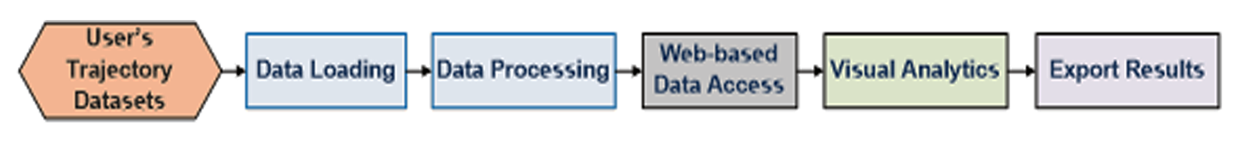
Thanks to advanced technologies in sensing and computing, the mobility patterns and dynamics of urban cities and their citizen are recorded and manifested in a variety of urban trajectory datasets, which include the moving paths of human, taxi, bus, fleets, cars, and so on. Understanding and analyzing such large-scale, complex data is of great importance to enhance both human lives and urban environments. TrajAnalytics provides exploratory data visualization tools for researchers, administrations, practitioners and general public to understand the data and to reveal knowledge intuitively.TrajAnalytics is a visual analytics software, which integrates scalable data management and interactive visualization with a powerful web-based computing platform. It contains two three major modules:
Trajectory Datasets and Data Types #back to top
A trajectory dataset consists of a set of trips. A trip refers to a trajectory in a specific period which is defined by users in the raw data. A trip includes a consecutive set of spatial sampling points, typically measured by its geolocation and timestamp.
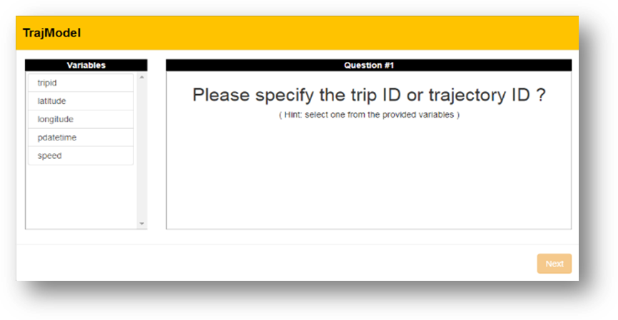
TrajAnalytics supports users to upload their raw trajectory datasets in CSV format with comma-separated values. Each data item refers to one sampling point. The values should include geolocations (longitude, latitude), trip ID, timestamp, and speed (optional). Here trip ID indicates which trip this point belongs to. Speed is optional.
Users can upload the raw CSV data through our data uploading interface. It will convert the raw data to a TD table, which is imported into our TrajBase database. TD table stores the trip data, instead of the raw sampling points. These points are aggregated by Trajectory ID into trips. TrajBase creates three types of spatial indices to enhance the query speed of data. The indices are B-Tree, GIST and Gin.A TD tables stores trips as groups of spatiotemporal points. However, they are not managed in the appropriate geographical context. TrajAnalytics further provides two different ways to match the trip data with geographical units, streets and regions, respectively.
TrajAnalytics provides a map-matching module for users to match their dataset with street network of the corresponding geographical area. The street network is automatically downloaded from OpenStreetMap, if available. A street network table is created in TrajBase which has a list of street segments each including a unique ID and the geometry (polylines) of the segment.A TDS tables stores trips similarly to a TD table, while in addition, a street ID links each point to a street segment.
When street network is not available or not to be used, TrajAnalytics supports map-matching of trips into spatial cells in the corresponding area. Currently, two types of cells are supported: Zipcode regions (US only) and grid cells. We found Zipcode regions are available freely in US only. So, we allow users to divide the area into a grid with arbitrary resolution, then match trips into the grid cells. In TrajBase, a region table of Zipcode regions or grid cells is created to store the list of cells each including a unique ID and the geometric boundaries of the regions/cells.A TDR tables store trips similarly to a TD table, while in addition, a region ID links each point to a geo region.
Data Loading and Processing Guide #back to top
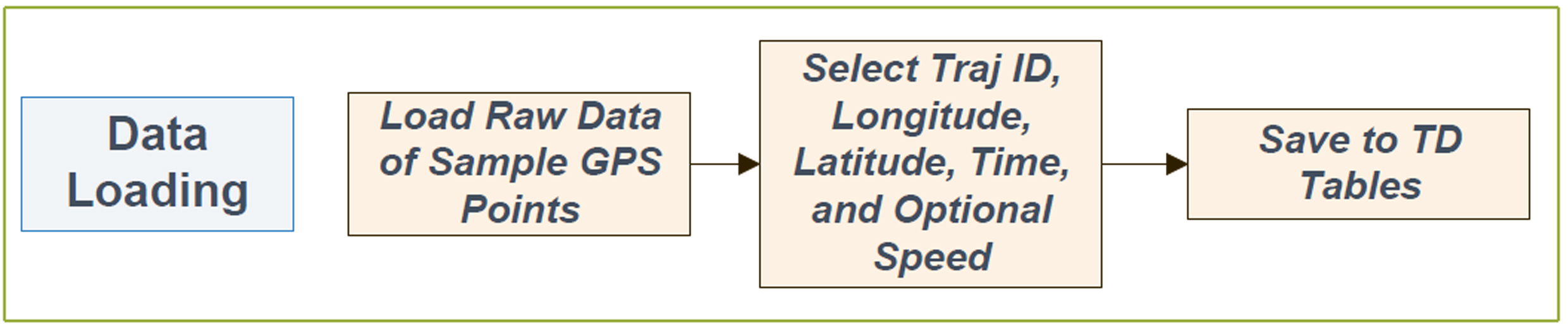
A trajectory dataset consists of a set of trips. A trip refers to a trajectory in a specific period which is defined by users in the raw data. A trip includes a consecutive set of spatial sampling points, typically measured by its geolocation and timestamp. TrajAnalytics supports users to upload their raw trajectory datasets in CSV format with comma-separated values. Each data item refers to one sampling point. The values should include geolocations (longitude, latitude), trip ID, timestamp, and speed (optional). Here trip ID indicates which trip this point belongs to. Speed is optional. The following steps shows the process of data loading.
Data Loading - #back to top
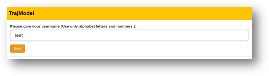
TrajAnalytics provides users with an independent data preprocessing module to load their own data to TrajAnalytics. This module can be accessed HERE.
- Input a user name
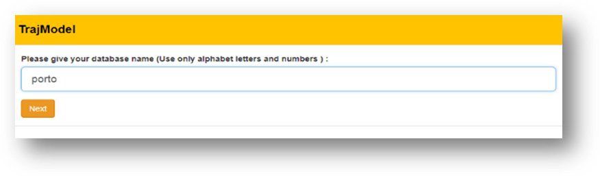
- Input a database name
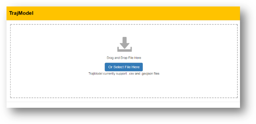
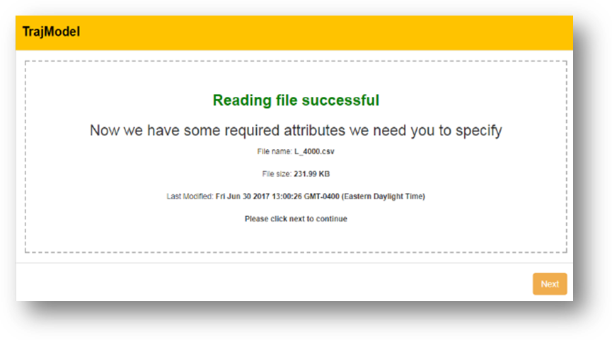
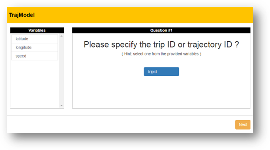
- Raw CSV file uploading
- Raw CSV file uploading
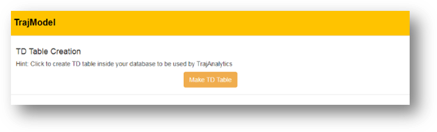
- Save TD tables
Street-Based Map Matching - #back to top
TrajAnalytics provides users with an independent data preprocessing module that automatically fetch corresponding road segments data from OpenStreetMap and match the raw GPS data with road segments. This module can be accessed HERE.
- Input the user name
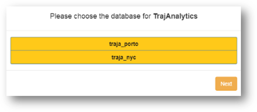
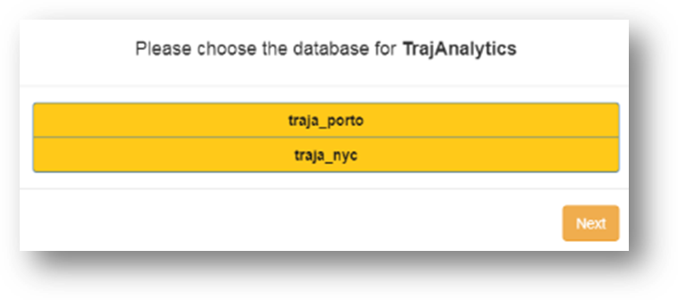
- Select the database
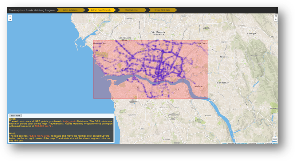
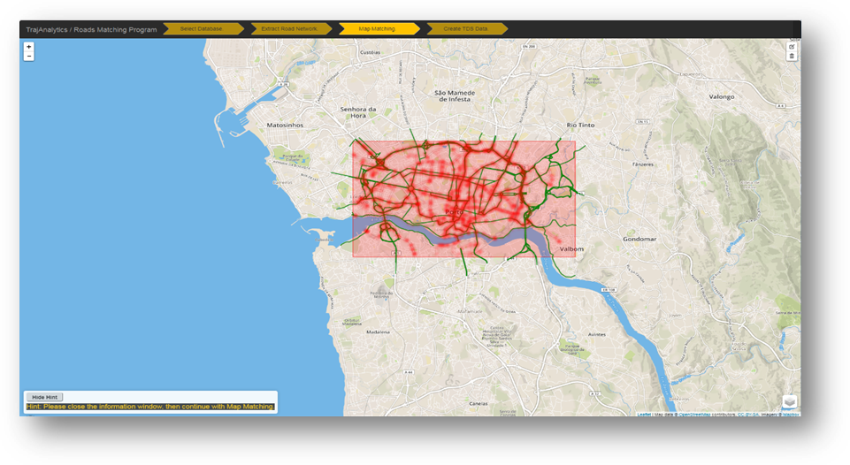
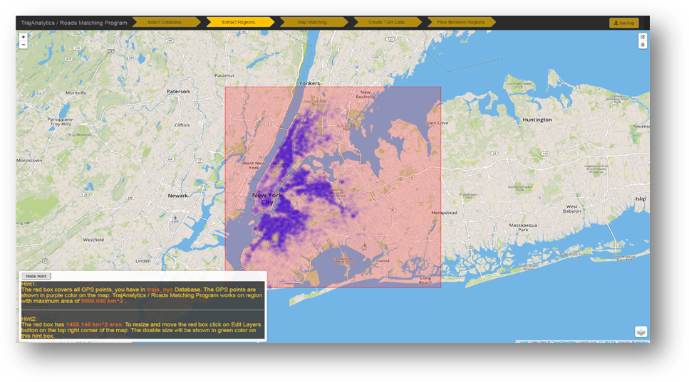
- Display heatmap and bounding box of all sample points
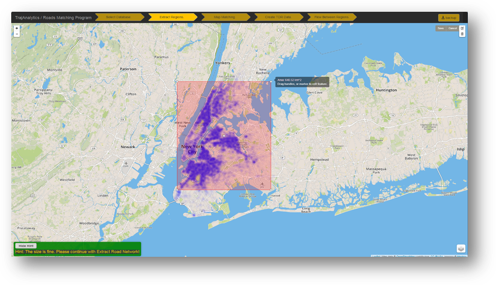
- User edit and select of working region bounding box
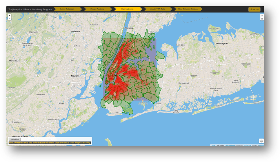
- Download street network from OSM
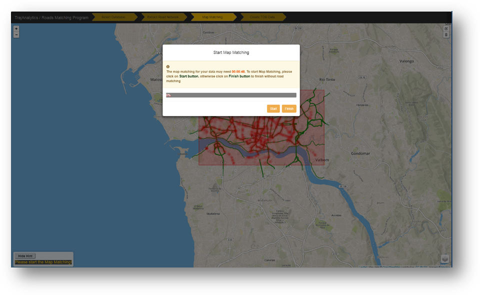
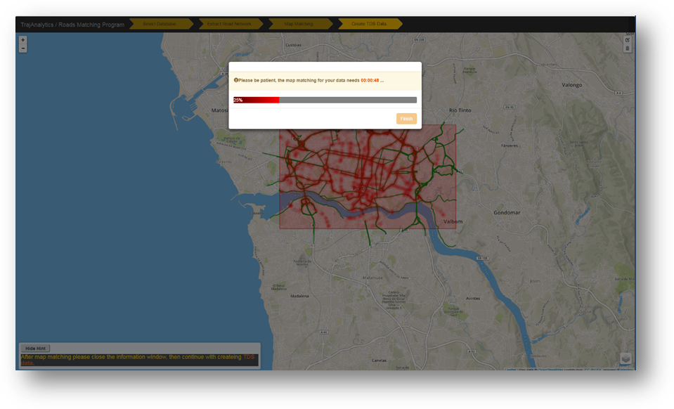
- Do Map Matching
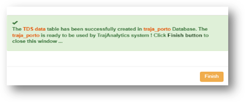
- Create TDS table in TrajBase


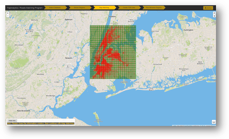
Region-Based Map Matching - #back to top
TrajAnalytics provides users with an independent data preprocessing module that automatically match the raw GPS data with regions (Zip code (USA Only) Regions, Grid). This module can be accessed HERE.
- Input the user name
- Select the database
- Display heatmap and bounding box of all sample points
- User edit and select of working region bounding box
- Zipcode based area division
- Grid based area division
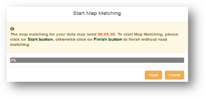
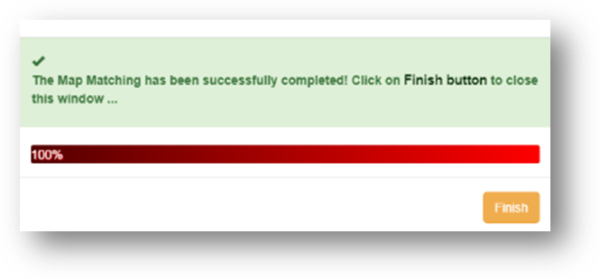
- Do Map Matching
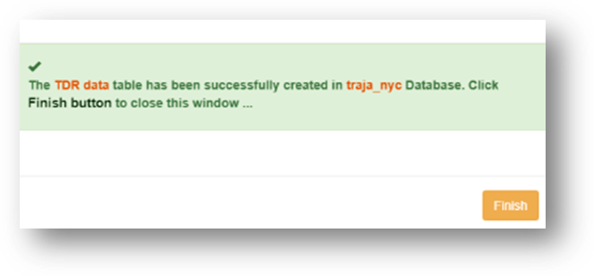
- Create TDR table in TrajBase

 A short video about how this software module works can be found below:
TrajAnalytics Account and Web-based Data Access #back to top
TrajAnalytics is a web-based cloud software. Users can upload the data and access it through their own account. The data will be stored for you only and will not be shared and published to other person or third parties. Please see our terms of services for details.
- Create TrajAnalytics accountCurrently, we are not open for online registration. If you would like to use TrajAnalytics, please send you request at vis.cs.kent.edu/registration
- Log in to access your account
- Access your data tables
After login, you will see the data tables you have uploaded and processed before.
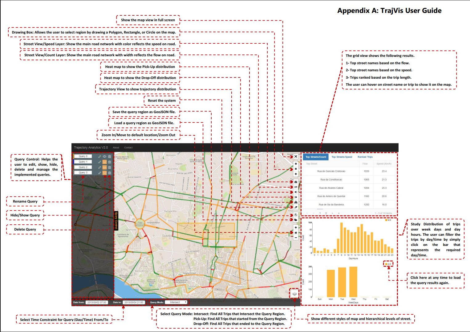
Visual Analytics Interface #back to top
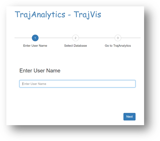
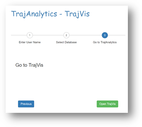
TrajVis is the web-based visual analytics interface of TrajAnalytics software. After users select the tables they would like to work on, TrajVis will prepare a set of visualization and interaction tools according to the types of data tables (TD, TDS, TDR). TrajVis can be accessed HERE.
- Input the user name
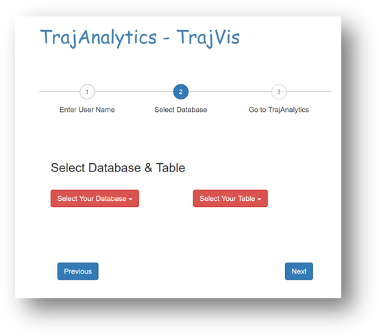
- Select the database and table
- Prepare a set of visualization and interaction tools according to the types of data tables (TD, TDS, TDR)
Spatiotemporal Query over TD, TDS or TDR data - #back to top
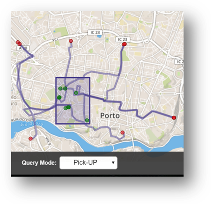
Users can query the loaded data table to retrieve trajectory data. The interface supports four types of spatial queries to specify a geometric area on the map. Meanwhile, users specify a time period. Then, users can query the trips starting from the specified area, or ending at the specified area, or traversing the specified area, or contained inside the specified area.
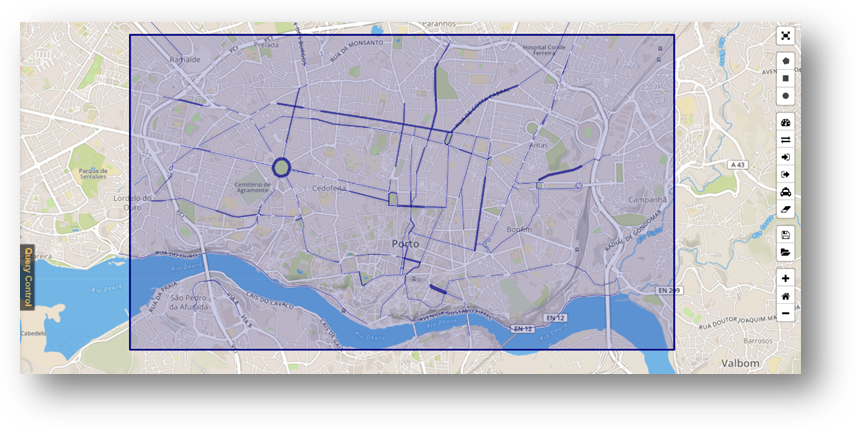
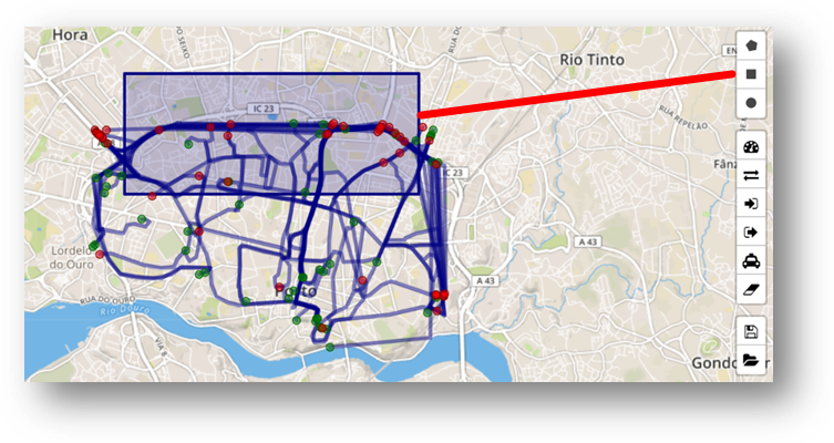
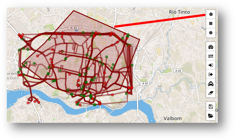
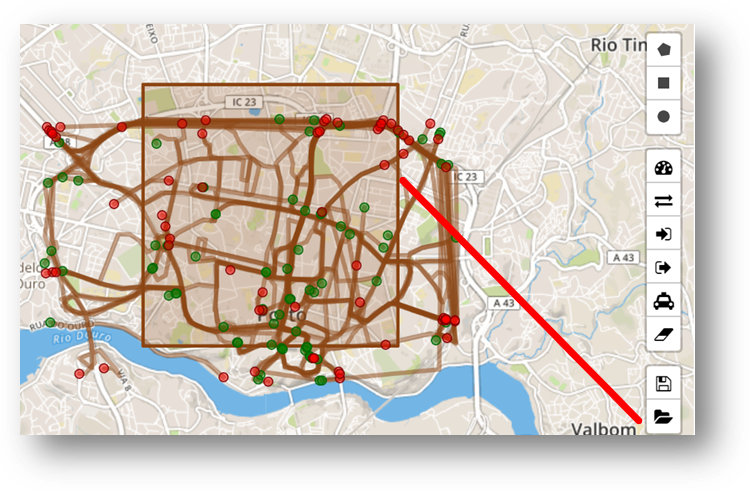
- Specify query area by pre-defined shapes from a file or drawing circle, rectangle, or polygon on the map
- Specify query time period
- Specify query conditions
- Query trips starting from the region
- Query trips ending at the region
- Query trips traversing region
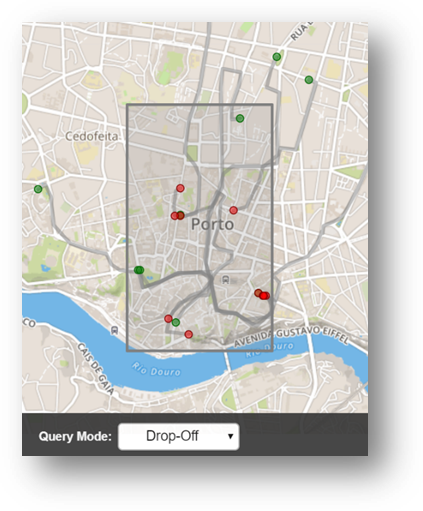
- Query Results
The query is transferred to TrajBase and all trips in the corresponding table is retrieved, processed and returned to TrajVis. With respect to different types of data tables, a set of attributes are computed and returned.
- Trip attributes
- The average speed of each trip
- The maximum speed of each trip
- The minimum speed of each trip
- Trip Start (origin) and end (destination) locations of each trip
- Street attributes (for TDS data)
- The average speed of all trips passing each street segment
- The maximum speed of all trips passing each street segment
- The minimum speed of all trips passing each street segment
- The number of trips (i.e. flow) passing each street segment
- Region attributes (for TDR data)
- The average speed of all trips passing each street segment
- The maximum speed of all trips passing each street segment
- The minimum speed of all trips passing each street segment
- The number of trips (i.e. flow) passing each street segment
- Time varying trip attributes
- Weekly averages of the attributes in the above V.B.1, such as the average speed of trips in Mondays, Tuesdays, …
- Hourly averages of the attributes in the above V.B.1, such as the average speed of trips in 8am, 10am, …
- Daily averages of the attributes in the above V.B.1 , such as the average speed of trips in each day in the specified time period.
- Time varying street attributes (for TDS data)
- Weekly averages of the attributes in the above V.B.3, such as the average speed of each street segment in Mondays, Tuesdays, …
- Hourly averages of the attributes in the above V.B.3, such as the average speed of each street segment in 8am, 10am, …
- Daily averages of the attributes in the above V.B.3, such as the average speed of each street segment in each day in the specified time period.
- Time varying region attributes (for TDR data)
- Weekly averages of the attributes in the above V.B.4, such as the average speed of each region in Mondays, Tuesdays, …
- Hourly averages of the attributes in the above V.B.4, such as the average speed of each region in 8am, 10am, …
- Daily averages of the attributes in the above V.B.4, such as the average speed of each region in each day in the specified time period.
- Trip attributes
- Visualization Query Results
The query results are shown in three different views: Map view, List view, Chart view.
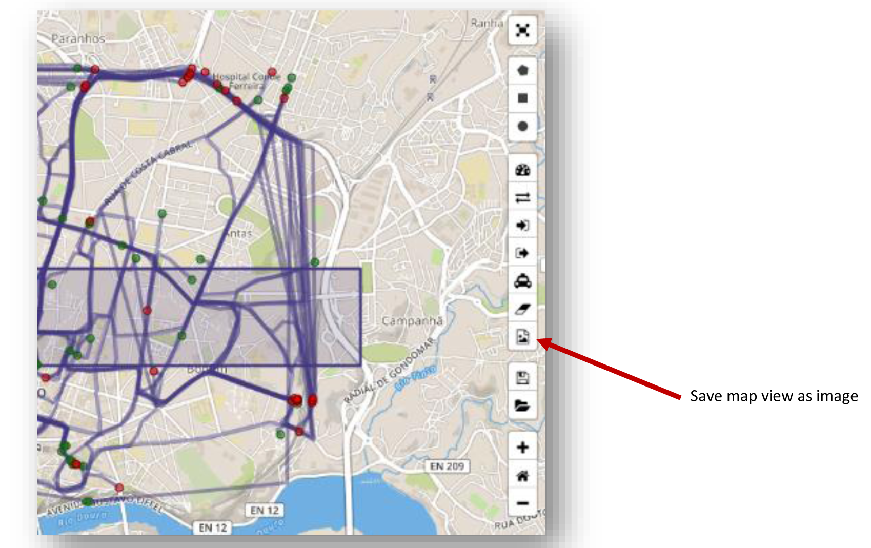
- Map view
There are several visualizations for users to select on how to show the query results:
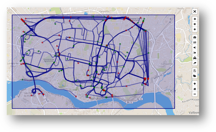
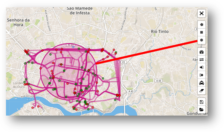
- Visualize trips
The trips are directly shown as connected polylines on the map. Users can select an attribute in V.B.1 to be visualized on each trip, which is represented by the line width and the color. The start and end locations in V.B.2 are visualized as red and green points, respectively.
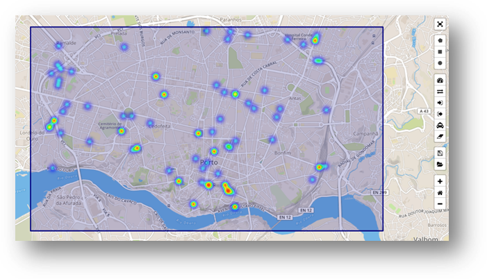
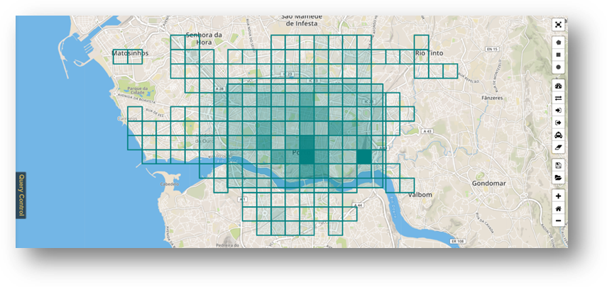
- Visualize heatmap of trip start and end locations
The start and end points in V.B.2 are aggregated and visualized as heatmap on the map. The density function of the colors represents the density of these points.
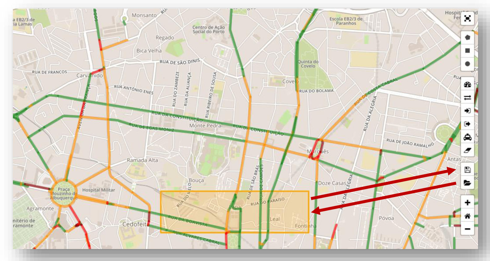
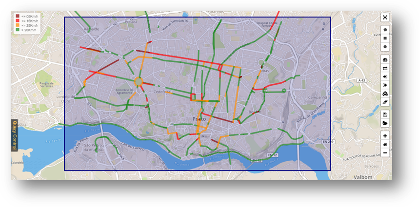
- Visualize attributes on streets (for TDS data)
The trips pass a group of roads. A set of attributes are computed on these roads by aggregating the information from these trips. Users can select an attribute in V.B.3 to be visualized on the street segments, which is represented by the line width of the streets, and the color of the streets.
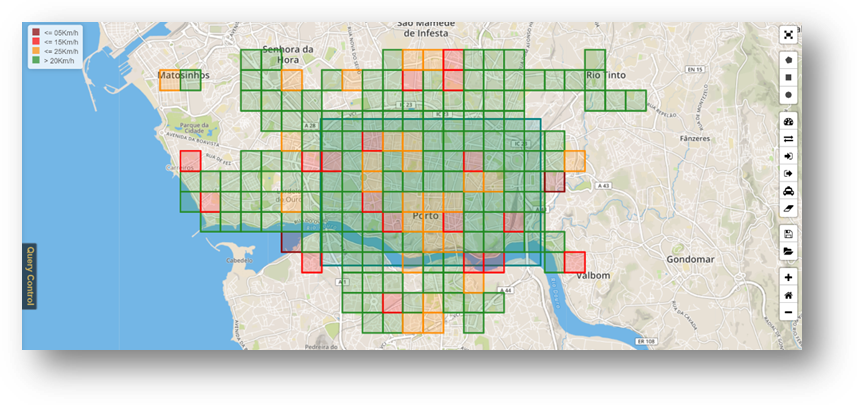
- Visualize attributes on regions (for TDR data)
Similarly, the trips pass a group of regions such as zipcode regions or grid cells. A set of attributes are computed on these regions by aggregating the information from these trips. Users can select one attribute in V.B.4 to be visualized on the zipcode regions or grid cells, which is represented by the color of these regions on the map.
- Visualize trips
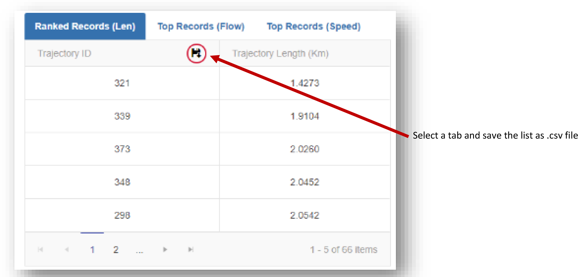
- List view
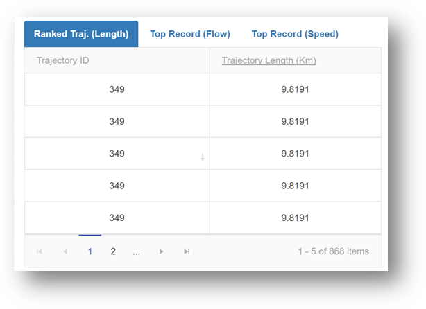
- Trip list
The trips are visualized in a maneuverable list with their attributes in V.B.1 as columns. Users can click on a column title to change the ranking order (descending or ascending) by the corresponding attribute.
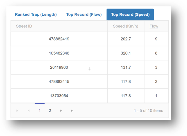
- Street list (for TDS data)
The streets are visualized in a maneuverable list with their attributes in V.B.3 as columns. Users can click on a column title to change the ranking order (descending or ascending) by the corresponding attribute.
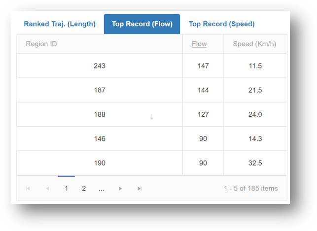
- Region list (for TDR data)
The regions are visualized in a maneuverable list with their attributes in V.B.4 as columns. Users can click on a column title to change the ranking order (descending or ascending) by the corresponding attribute.
- Trip list
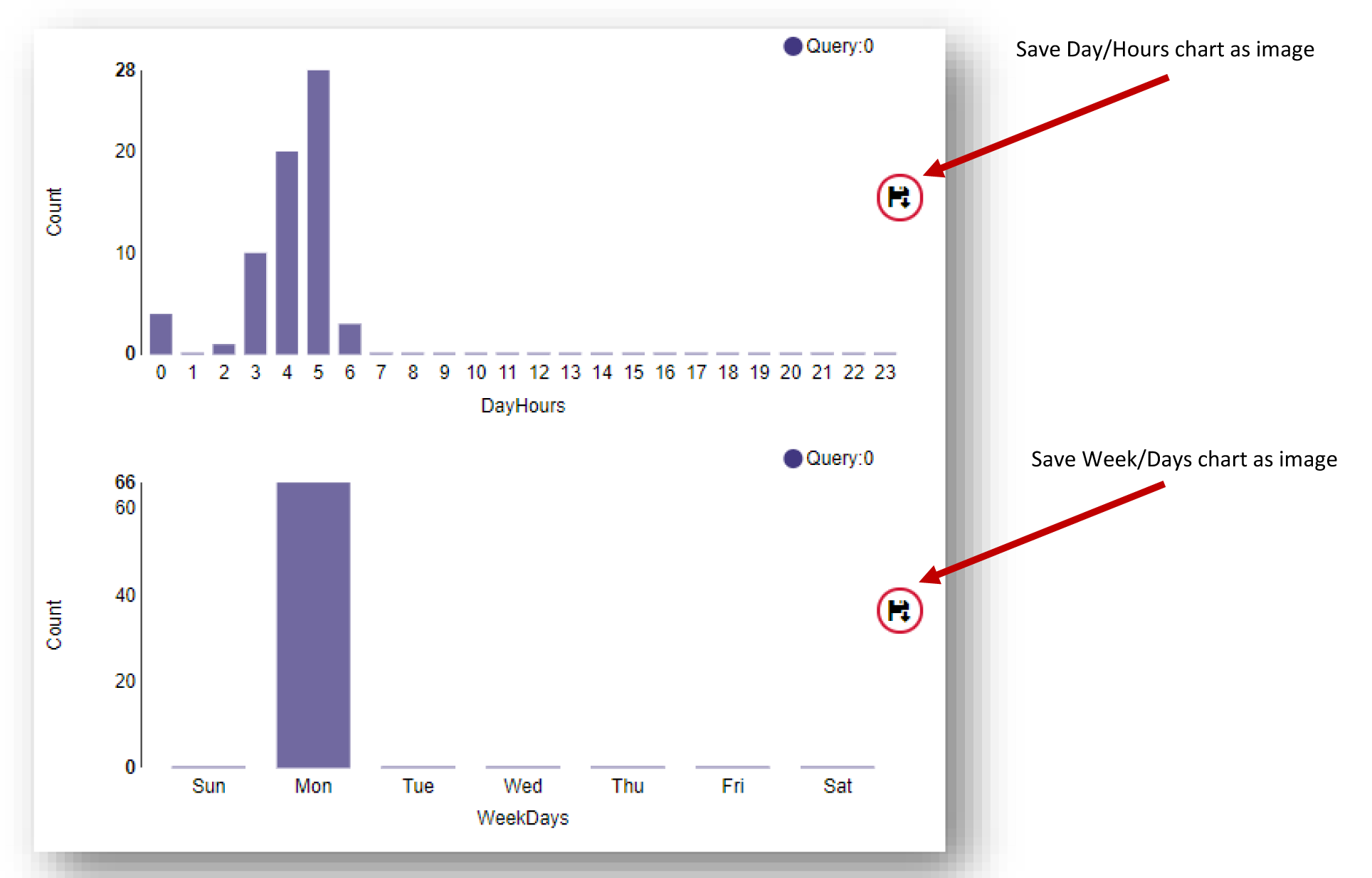
- Chart view
The trips are distributed in the given time period. Three types of charts are used to visualize the facts related to time windows.
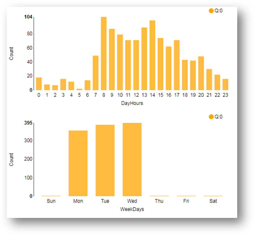
- Weekly chart
- Trips: The attributes in V.B.5 are visualized in the bar charts along different weekdays of weeks.
- Streets (for TDS data): The attributes in V.B.6 are visualized in the bar charts along different weekdays of weeks.
- Regions (for TDR data): The attributes in V.B.7 are visualized in the bar charts along different weekdays of weeks.
- Hourly chart
- Trips: The attributes in V.B.5 are visualized in the bar charts along different hours of weeks.
- Streets (for TDS data): The attributes in V.B.6 are visualized in the bar charts along different hours of weeks.
- Regions (for TDR data): The attributes in V.B.7 are visualized in the bar charts along different hours of weeks.
- Daily chart
- Trips: The attributes in V.B.5 are visualized in the bar charts along different days of weeks.
- Streets (for TDS data): The attributes in V.B.6 are visualized in the bar charts along different days of weeks.
- Regions (for TDR data): The attributes in V.B.7 are visualized in the bar charts along different days of weeks.
- Weekly chart
- Map view

Result Saving and Report #back to top
- Save Query Results for Reuse and Sharing
- Save Visualization Results
- Save charts as image
- Save lists as (.csv) file
- Save map view as image